Reflectance equation
这里采用的反射模型如下:
$$ L_o(p,\omega_o) = \int_\Omega (k_d \frac{c}{\pi} + k_s \frac{DFG}{4(\omega_o \cdot n)(\omega_i \cdot n)})L_i(p,\omega_i)(n \cdot \omega_i) d\omega_i $$ $$ \Rightarrow L_o(p,\omega_i) = \int_\Omega k_d \frac{c}{\pi}L_i(p,\omega_i)n\cdot \omega_i d\omega_i + \int_\Omega k_s \frac{DFG}{4(\omega_i \cdot n)(\omega_o \cdot n)}L_i(p,\omega_i)(n \cdot \omega_i) d\omega_i $$Diffuse Irradiance
接下来先看diffuse项:
$$ L_o = \int_\Omega k_d\frac{c}{\pi}L_i(p,\omega_i) (n \cdot \omega_i ) d\omega_i $$ $$ \Rightarrow L_o = k_d\frac{c}{\pi}\int_\Omega L_i(p,\omega_i) (n\cdot \omega_i) d\omega_i $$ $$ \Rightarrow L_o = k_d \frac{c}{\pi}\int_{\phi = 0}^{2\pi} \int_{\theta = 0}^{\frac{\pi}{2}}L_i(p,\phi_i,\theta_i)\cos(\theta)\sin(\theta)d\phi d\theta \tag{1} $$蒙特卡洛方法
$$ \because E[\frac{f(x)}{p(x)}] = \int f(x)dx $$设$\frac{f(x_1)}{p(x_1)},\frac{f(x_2)}{p(x_2)},...,\frac{f(x_n)}{p(x_n)}$为独立同分布的随机变量,因此构造估计量如下:
$$ \sigma = \frac{1}{N}\sum_{i=0}^{N} \frac{f(x_i)}{p(x_i)} $$根据大数定律得知,样本均值将会收敛于期望值,因此当N增大,估计量将会逐渐逼近于期望$\int f(x)dx$
接下来证明下无偏性:
$$ E[\sigma] = E[\frac{1}{N}\sum_{i=0}^{N} \frac{f(x_i)}{p(x_i)}] $$ $$ \Rightarrow E[\sigma] = \frac{1}{N}E[\sum_{i = 0}^{N}\frac{f(x_i)}{p(x_i)}] $$ $$ \Rightarrow E[\sigma] = \frac{1}{N}\sum_{i = 0}^{N}E[\frac{f(x_i)}{p(x_i)}] $$ $$ \Rightarrow E[\sigma] = \frac{1}{N}NE[\frac{f(x)}{p(x)}] = \int f(x)dx $$接下来使用蒙特卡洛方法来分解方程(1),使用均匀分布$p(\phi) = \frac{1}{2\pi},p(\theta) = \frac{1}{(\frac{\pi}{2})} = \frac{2}{\pi}$
构造估计量如下:
$$ L_o = k_d \frac{c}{\pi}\frac{1}{n_1}\frac{1}{n_2}\sum_{i = 1}^{n_1}\sum_{j = 1}^{n_2}\frac{L_i(p,\phi_i,\theta_j)cos(\theta_j)sin(\theta_j)}{p(\phi)\cdot p(\theta)}d\phi d\theta $$ $$ \Rightarrow L_o = k_d\frac{c}{\pi}\frac{1}{n_1 n_2} 2\pi \frac{\pi}{2}\sum_{i = 1}^{n_1}\sum_{j = 1}^{n_2}L_i(p,\phi_i,\theta_j)cos(\theta_j)\sin(\theta_j)d\phi d\theta $$ $$ \Rightarrow L_o = k_d c\frac{\pi}{n_1 n_2}\sum_{i = 1}^{n_1}\sum_{j = 1}^{n_2}L_i(p,\phi_i,\theta_j)cos(\theta_j)\sin(\theta_j)d\phi d\theta $$实现就显得很简单了,IBL中贴图的每个texel都是一个光源,即提供了$L_i$的数据,代码如下:
1 | int phiSampleCount = 100; |
以如下环境贴图为例: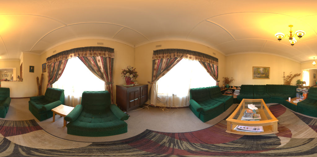
Irradiance Map如下:
Specular IBL
对Specular项应用蒙特卡洛积分:
$$ \int_\Omega L_i(p,\omega_i)f(p,\omega_i,\omega_o)(n \cdot \omega_i) d\omega_i \approx \frac{1}{N}\sum_{k = 1}^N\frac{L_i(p,\omega_{i})f(p,\omega_{i},\omega_{o})(n\cdot \omega_{i})}{pdf} $$UE4中对其进行了一个近似,划分成了两个累加的乘积:
$$ \frac{1}{N}\sum_{k = 1}^N\frac{L_i(p,\omega_{i})f(p,\omega_{i},\omega_{o})(n\cdot \omega_{i})}{pdf} \approx \Big(\frac{1}{N}\sum_{k = 1}^N L_i(p,\omega_{i}\Big )\Big (\frac{1}{N}\sum_{k = 1}^{N}\frac{f(p,\omega_{i}, \omega_{o})(n \cdot \omega_{i})}{pdf}\Big ) $$Pre-Filtered Environment Map
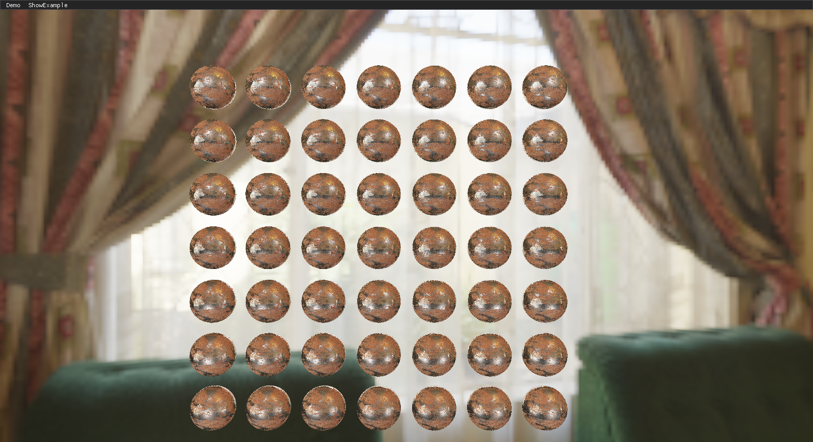
对于第一个累加,常用的方案是使用GGX的重要性采样对环境贴图进行卷积计算
我们可以针对不同的粗糙度值进行预计算,并将结果保存在mipmap中
由于使用了微表面模型,分布的形状将会受到视角的影响,因此,这里假定为各向同性,即$N = V = R$
但这也意味着我们从与法线垂直的方向去看表面,无法得到强烈的反射,针对这一点,使用$\cos(\omega_i)$进行加权解决
实现如下:
1 | for (int miplevel = 0; miplevel < mipNum; miplevel++) |
计算结果如下: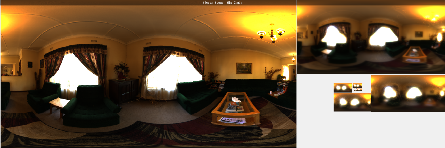
Precompute BRDF LUT
接着分解第二个累加项:
$$ \frac{1}{N}\sum_{k = 1}^{N}\frac{f(p,\omega_{i}, \omega_{o})(n \cdot \omega_{i})}{pdf} = \frac{1}{N}\sum_{k = 1}^{N}\frac{f(p,\omega_{i}, \omega_{o})(n \cdot \omega_{i}) \times F(\omega_{o},\omega_h)}{pdf \times F(\omega_{o},\omega_h)} $$ $$ \because F(\omega_o, \omega_h) = F_0 + (1 - F_0)(1 - \omega_o \cdot \omega_h)^5 $$ $$ \Rightarrow \frac{1}{N}\sum_{k = 1}^{N}\frac{f(p,\omega_{i}, \omega_{o})(n \cdot \omega_{i}) \times (F_0 (1 - (1 - \omega_{o} \cdot \omega_h)^5) + (1 - \omega_{o} \cdot \omega_h)^5)}{pdf \times F(\omega_{o},\omega_h)} $$ $$ \Rightarrow \frac{F_0}{N}\sum_{k = 1}^{N} \frac{f(p,\omega_{i}, \omega_{o})(n\cdot \omega_{i}) \times (1 - (1 - \omega_{o} \cdot \omega_h)^5)}{pdf \times F(\omega_{o}, \omega_h)} + \\\\ \frac{1}{N}\sum_{k = 1}^{N}\frac{f(p,\omega_{i},\omega_{o}) (n\cdot \omega_{i}) \times (1 - \omega_{o} \cdot \omega_h)^5}{pdf \times F(\omega_{o},\omega_h)} \tag{2} $$由于我们使用的是微表面模型:
$$ f(p,\omega_i,\omega_o) = \frac{D(\omega_h)F(\omega_o,\omega_h)G(\omega_i,\omega_o)}{4(\omega_i \cdot n)(\omega_o \cdot n)} $$GGX重要性采样的PDF为:
$$ pdf = \frac{D(\omega_h)(\omega_h \cdot n)}{4 (\omega_o \cdot \omega_h)} $$因此:
$$ \frac{f(p,\omega_i,\omega_o)(\omega_i \cdot n)}{pdf \times F(\omega_o,\omega_h)} = \frac{D(\omega_h)F(\omega_o,\omega_h)G(\omega_i,\omega_o)(\omega_i \cdot n)}{4(\omega_i \cdot n)(\omega_o \cdot n)} \times \frac{4 (\omega_o \cdot \omega_h)}{D(\omega_h)(\omega_h \cdot n) F(\omega_o,\omega_h)} $$ $$ \Rightarrow = \frac{G(\omega_i,\omega_o)(\omega_o \cdot \omega_h)}{(\omega_o \cdot n)(\omega_h \cdot n)} $$代入(2)式可得:
$$ \frac{F_0}{N}\sum_{k = 1}^N \frac{G(\omega_i,\omega_o)(\omega_o \cdot \omega_h)(1 - (1 - \omega_o \cdot n)^5)}{(\omega_o \cdot n)(\omega_h \cdot n)} + \frac{1}{N}\sum_{k = 1}{N}\frac{G(\omega_i,\omega_o)(\omega_o \cdot \omega_h) (1 - \omega_o \cdot h)^5}{(\omega_o \cdot n)(\omega_h \cdot n)} $$因此可以以roughness与$(\omega_o \cdot n)$作为变量来预计算上述方程,以roughness,$(\omega_o \cdot n)$为行列得到预计算的BRDF查找表
代码如下:
1 | SVector2f IntegrateBRDF(float roughness, float NdotV) |
预计算结果如下:
最终Specular IBL计算如下:
1 | float3 irradiance = IrradianceMap.Sample(samplerIrradiace, CartesianToSpherical(N)).rgb; |
实现代码可参考这里,效果如下: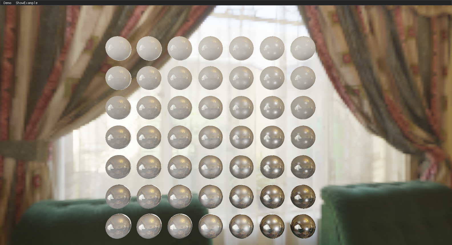
Comments